Supervised learning

  Support Vector Machine Support vector machine (SVM) is one of the most popular algorithms in machine learning. It is a powerful supervised...

 

Support Vector Machine

Support vector machine (SVM) is one of the most popular algorithms in machine learning. It is a powerful supervised algorithm used for classification, regression, and outlier detection.

SVM has many applications in investment management. It is particularly suited for small to medium-size but complex high-dimensional datasets, such as corporate financial statements or bankruptcy databases. Investors seek to predict company failures for identifying stocks to avoid or to short sell, and SVM can generate a binary classification (e.g., bankruptcy likely versus bankruptcy unlikely) using many fundamental and technical feature variables. SVM can effectively capture the characteristics of such data with many features while being resilient to outliers and correlated features. SVM can also be used to classify text from documents (e.g., news articles, company announcements, and company annual reports) into useful categories for investors (e.g., positive sentiment and negative sentiment).

Despite its complicated-sounding name, the notion is relatively straightforward and best explained with a few pictures.

Scatterplots and Linear Separation of Labeled Data

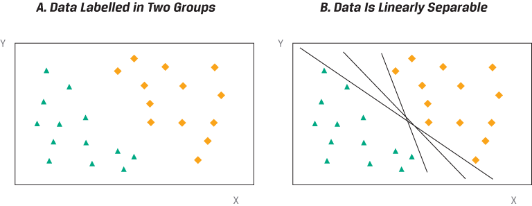
Linear Support Vector Machine Classifier

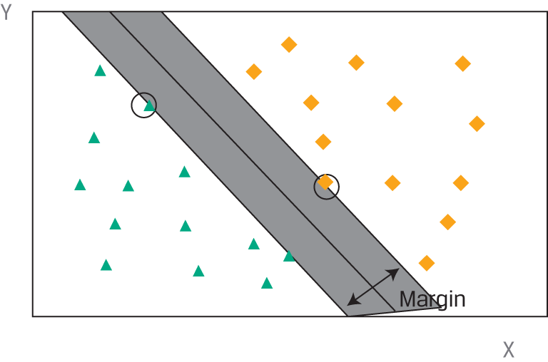
In the example above, SVM is classifying all observations perfectly. Most real-world datasets, however, are not linearly separable. Some observations may fall on the wrong side of the boundary and be misclassified by the SVM algorithm. The SVM algorithm handles this problem by an adaptation called soft margin classification, which adds a penalty to the objective function for observations in the training set that are misclassified. In essence, the SVM algorithm will choose a discriminant boundary that optimizes the trade-off between a wider margin and a lower total error penalty.

As an alternative to soft margin classification, a non-linear SVM algorithm can be run by introducing more advanced, non-linear separation boundaries. These algorithms may reduce the number of misclassified instances in the training datasets but are more complex and, so, are prone to overfitting.

K-Nearest Neighbor

K-nearest neighbor (KNN) is a supervised learning technique used most often for classification and sometimes for regression. The idea is to classify a new observation by finding similarities (“nearness”) between this new observation and the existing data.

The KNN algorithm has many applications in the investment industry, including bankruptcy prediction, stock price prediction, corporate bond credit rating assignment, and customized equity and bond index creation. For example, KNN is useful for determining bonds that are similar and those that are dissimilar, which is critical information for creating a custom, diversified bond index.

Scatterplots and Linear Separation of Labeled Data.

Referencing the scatterplot above, let us assume we have a new observation: The diamond in the scatterplot below needs to be classified as belonging to either the cross or the triangle category. Click on each information icon to find out more.

K-Nearest Neighbor Algorithm

Let us suppose we have a database of corporate bonds classified by credit rating that also contains detailed information on the characteristics of these bonds. Such features would include those of the issuing company (e.g., asset size, industry, leverage ratios, cash flow ratios) and of the bond issue itself (e.g., tenor, fixed/floating coupon, embedded options). Now, assume a new bond is about to be issued with no credit rating. By nature, corporate bonds with similar issuer and issue characteristics should be given a similar credit rating. So, by using KNN, we can predict the implied credit rating of the new bond based on the similarities of its characteristics to those of the bonds in our database.

KNN is a straightforward, intuitive model that is still very powerful because it is non-parametric; the model makes no assumptions about the distribution of the data. Moreover, it can be used directly for multi-class classification. A critical challenge of KNN, however, is defining what it means to be “similar” (or near). Besides the selection of features, an important decision relates to the distance metric used to model similarity because an inappropriate measure will generate poorly performing models. The choice of a correct distance measure may be even more subjective for ordinal or categorical data. For example, if an analyst is looking at the similarities in market performance of various equities, he or she may consider using the correlation between the stocks’ historical returns as an appropriate measure of similarity.

Knowledge of the data and understanding of the business objectives of the analysis are critical aspects in the process of defining similarity. KNN results can be sensitive to inclusion of irrelevant or correlated features, so it may be necessary to select features manually. By doing so, the analyst removes less valuable information to keep the most relevant and pertinent information. If done correctly, this process should generate a more representative distance measure. KNN algorithms tend to work better with a small number of features.

Finally, the number k, the hyperparameter of the model, must be chosen with the understanding that different values of k can lead to different conclusions. For predicting the credit rating of an unrated bond, for example, should k be the 3, 15, or 50 bonds most similar to the unrated bond? If k is an even number, there may be ties and no clear classification. Choosing a value for k that is too small would result in a high error rate and sensitivity to local outliers, but choosing a value for k that is too large would dilute the concept of nearest neighbors by averaging too many outcomes. In practice, several different techniques can be used to determine an optimal value for k, taking into account the number of categories and their partitioning of the feature space.

Classification and Regression Tree

Classification and regression tree (CART) is another common supervised machine learning technique that can be applied to predict either a categorical target variable, producing a classification tree, or a continuous target variable, producing a regression tree. CART is commonly applied to binary classification or regression.

CART models are popular supervised machine learning models because the tree provides a visual explanation for the prediction. This contrasts favorably with other algorithms that are often considered to be “black boxes” because it may be difficult to understand the reasoning behind their outcomes and thus to place trust in them. CART is a powerful tool to build expert systems for decision-making processes. It can induce robust rules despite noisy data and complex relationships between high numbers of features. Typical applications of CART in investment management include, among others, enhancing detection of fraud in financial statements, generating consistent decision processes in equity and fixed-income selection, and simplifying communication of investment strategies to clients.

CART is discussed here in the context of a simplified model for classifying companies by whether they are likely to increase their dividends to shareholders.

Classification and Regression Tree—Decision Tree and Partitioning of the Feature Space

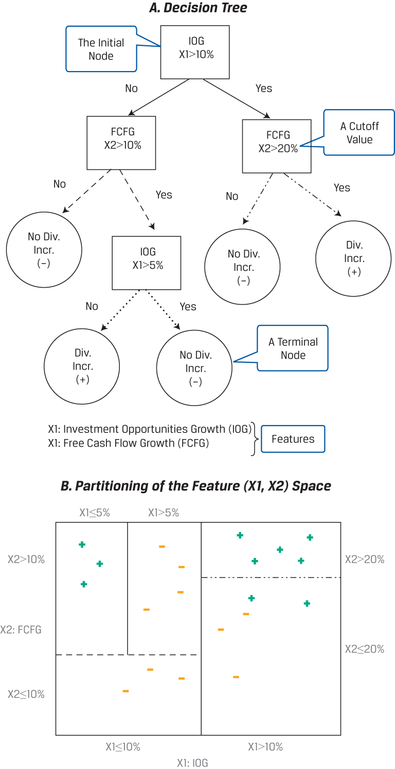
Such a classification requires a binary tree: a combination of an initial root node, decision nodes, and terminal nodes. The root node and each decision node represent a single feature (f) and a cutoff value (c) for that feature. As shown in Panel A, we start at the initial root node for a new data point. In this case, the initial root node represents the feature investment opportunities growth (IOG), designated as X1, with a cutoff value of 10%. From the initial root node, the data are partitioned at decision nodes into smaller and smaller subgroups until terminal nodes that contain the predicted labels are formed. In this case, the predicted labels are either dividend increase (the cross) or no dividend increase (the dash).

Also shown in Panel A, if the value of feature IOG (X1) is greater than 10% (Yes), then we proceed to the decision node for free cash flow growth (FCFG), designated as X2, which has a cutoff value of 20%. Now, if the value of FCFG is not greater than 20% (No), then CART will predict that that data point belongs to the no dividend increase (dash) category, which represents a terminal node. Conversely, if the value of X2 is greater than 20% (Yes), then CART will predict that that data point belongs to the dividend increase (cross) category, which represents another terminal node.

It is important to note that the same feature can appear several times in a tree in combination with other features. Moreover, some features may be relevant only if other conditions have been met. For example, going back to the initial root node, if IOG is not greater than 10% (X1 ≤ 10%) and FCFG is greater than 10%, then IOG appears again as another decision node, but this time it is lower down in the tree and has a cutoff value of 5%.

We now turn to how the CART algorithm selects features and cutoff values for them. Initially, the classification model is trained from the labeled data, which in this hypothetical case are 10 instances of companies having a dividend increase (the crosses) and 10 instances of companies with no dividend increase (the dashes). As shown in Panel B, at the initial root node and at each decision node, the feature space (i.e., the plane defined by X1 and X2) is split into two rectangles for values above and below the cutoff value for the particular feature represented at that node. This can be seen by noting the distinct patterns of the lines that emanate from the decision nodes in Panel A. These same distinct patterns are used for partitioning the feature space in Panel B.

The CART algorithm chooses the feature and the cutoff value at each node that generates the widest separation of the labeled data to minimize classification error (e.g., by a criterion, such as mean-squared error). After each decision node, the partition of the feature space becomes smaller and smaller, so observations in each group have lower within-group error than before. At any level of the tree, when the classification error does not diminish much more from another split (bifurcation), the process stops, the node is a terminal node, and the category that is in the majority at that node is assigned to it. If the objective of the model is classification, then the prediction of the algorithm at each terminal node will be the category with the majority of data points. For example, in Panel B, the top right rectangle of the feature space, representing IOG (X1) > 10% and FCFG (X2 )> 20%, contains five crosses, the most data points of any of the partitions. So, CART would predict that a new data point (i.e., a company) with such features belongs to the dividend increase (cross) category. However, if instead the new data point had IOG (X1) > 10% and FCFG (X2) ≤ 20%, then it would be predicted to belong to the no dividend increase (dash) category—represented by the lower right rectangle, with two crosses but with three dashes. Finally, if the goal is regression, then the prediction at each terminal node is the mean of the labeled values.

CART makes no assumptions about the characteristics of the training data, so if left unconstrained, it potentially can perfectly learn the training data. To avoid such overfitting, regularization parameters can be added, such as the maximum depth of the tree, the minimum population at a node, or the maximum number of decision nodes. The iterative process of building the tree is stopped once the regularization criterion has been reached. For example, in Panel B, the upper left rectangle of the feature space (determined by X1 ≤ 10%, X2 > 10%, and X1 ≤ 5% with three crosses) might represent a terminal node resulting from a regularization criterion with minimum population equal to 3. Alternatively, regularization can occur via a pruning technique that can be used afterward to reduce the size of the tree. Sections of the tree that provide little classifying power are pruned (i.e., cut back or removed).

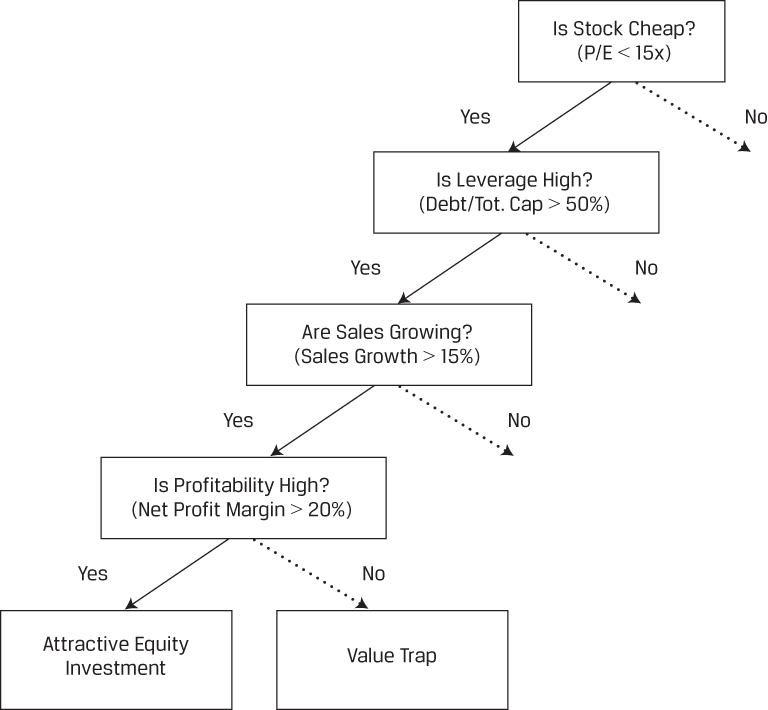
By its iterative structure, CART can uncover complex dependencies between features that other models cannot reveal. As demonstrated in above, the same feature can appear several times in combination with other features and some features may be relevant only if other conditions have been met.

As shown in the tree below, high profitability is a critical feature for predicting whether a stock is an attractive investment or a value trap (i.e., an investment that, although apparently priced cheaply, is likely to be unprofitable). This feature is relevant only if the stock is cheap: For example, in this hypothetical case, if P/E is less than 15, leverage is high (debt to total capital > 50%) and sales are expanding (sales growth > 15%). Said another way, high profitability is irrelevant in this context if the stock is not cheap and if leverage is not high and if sales are not expanding. Multiple linear regression typically fails in such situations where the relationship between the features and the outcome is non-linear.

Stylized Decision Tree—Attractive Investment or Value Trap?

Ensemble Learning and Random Forest

Instead of basing predictions on the results of a single model as in the previous discussion, why not use the predictions of a group—or an ensemble—of models? Each single model will have a certain error rate and will make noisy predictions. But by taking the average result of many predictions from many models, we can expect to achieve a reduction in noise as the average result converges toward a more accurate prediction. This technique of combining the predictions from a collection of models is called ensemble learning, and the combination of multiple learning algorithms is known as the ensemble method. Ensemble learning typically produces more accurate and more stable predictions than the best single model. In fact, in many prestigious machine learning competitions, an ensemble method is often the winning solution.

Ensemble learning can be divided into two main categories: (1) aggregation of heterogeneous learners (i.e., different types of algorithms combined with a voting classifier) or (2) aggregation of homogeneous learners (i.e., a combination of the same algorithm using different training data that are based, for example, on a bootstrap aggregating, or bagging, technique, as discussed later).

Voting Classifiers

Suppose you have been working on a machine learning project for some time and have trained and compared the results of several algorithms, such as SVM, KNN, and CART. A majority-vote classifierwill assign to a new data point the predicted label with the most votes. For example, if the SVM and KNN models are both predicting the category “stock outperformance” and the CART model is predicting the category “stock underperformance,” then the majority-vote classifier will choose stock outperformance.” The more individual models you have trained, the higher the accuracy of the aggregated prediction up to a point. There is an optimal number of models beyond which performance would be expected to deteriorate from overfitting. The trick is to look for diversity in the choice of algorithms, modeling techniques, and hypotheses. The (extreme) assumption here is that if the predictions of the individual models are independent, then we can use the law of large numbers to achieve a more accurate prediction.

Bootstrap Aggregating (Bagging)

Alternatively, one can use the same machine learning algorithm but with different training data. Bootstrap aggregating (or bagging) is a technique whereby the original training dataset is used to generate n new training datasets or bags of data. Each new bag of data is generated by random sampling with replacement from the initial training set. The algorithm can now be trained on nindependent datasets that will generate n new models. Then, for each new observation, we can aggregate the n predictions using a majority-vote classifier for a classification or an average for a regression. Bagging is a very useful technique because it helps to improve the stability of predictions and protects against overfitting the model.

Random Forest

A random forest classifier is a collection of a large number of decision trees trained via a bagging method. For example, a CART algorithm would be trained using each of the n independent datasets (from the bagging process) to generate the multitude of different decision trees that make up the random forest classifier.

To derive even more individual predictions, added diversity can be generated in the trees by randomly reducing the number of features available during training. So, if each observation has n features, one can randomly select a subset of m features (where m < n) that will then be considered by the CART algorithm for splitting the dataset at each of the decision nodes. The number of subset features (m), the number of trees to use, the minimum size (population) of each node (or leaf), and the maximum depth of each tree are all hyperparameters that can be tuned to improve overall model prediction accuracy. For any new observation, we let all the classifier trees (the “random forest”) undertake classification by majority vote—implementing a machine learning version of the “wisdom of crowds.” The process involved in random forest construction tends to reduce variance and protect against overfitting on the training data. It also reduces the ratio of noise to signal because errors cancel out across the collection of slightly different classification trees. However, an important drawback of random forest is that it lacks the ease of interpretability of individual trees; as a result, it is considered a relatively black box type of algorithm.

Scatterplots

In the graph below, we have three scatterplots of actual and predicted defaults by small and medium-sized businesses with respect to two features, X and Y—for example, firm profitability and leverage, respectively. Click on each plot to find out more.

Credit Defaults of Small- and Medium-Sized Borrowers

Ensemble Learning with Random Forest

In making use of voting across classifier trees, random forest is an example of ensemble learning: Incorporating the output of a collection of models produces classifications that have better signal-to-noise ratios than the individual classifiers. A good example is a credit card fraud detection problem that comes from an open source dataset on Kaggle.¹ Here, the data contained several anonymized features that might be used to explain which transactions were fraudulent. The difficulty in the analysis arises from the fact that the rate of fraudulent transactions is very low; in a sample of 284,807 transactions, only 492 were fraudulent (0.17%). This is akin to finding a needle in a haystack. Applying a random forest classification algorithm with an oversampling technique—which involves increasing the proportional representation of fraudulent data in the training set—does extremely well. Despite the lopsided sample, it delivers precision (the ratio of correctly predicted fraudulent cases to all predicted fraudulent cases) of 89% and recall (the ratio of correctly predicted fraudulent cases to all actual fraudulent cases) of 82%.

Despite its relative simplicity, random forest is a powerful algorithm with many investment applications. These include, for example, use in factor-based investment strategies for asset allocation and investment selection or use in predicting whether an IPO will be successful (e.g., percent oversubscribed, first trading day close/IPO price) given the attributes of the IPO offering and the corporate issuer. Later, in a mini-case study, Deep Neural Network–Based Equity Factor Model, we present further details of how supervised machine learning is used for fundamental factor modeling.

Case Study: Classification of Winning and Losing Funds

The following case study was developed and written by Matthew Dixon, PhD, FRM. You can access the Python code that was used to develop this case study at the end of this lesson.

A research analyst for a fund of funds has been tasked with identifying a set of attractive exchange-traded funds (ETFs) and mutual funds (MFs) in which to invest. She decides to use machine learning to identify the best (i.e., winners) and worst (i.e., losers) performing funds and the features which are most important in such an identification. Her aim is to train a model to correctly classify the winners and losers and then to use it to predict future outperformers. She is unsure of which type of machine learning classification model (i.e., classifier) would work best, so she reports and cross-compares her findings using several different well-known machine learning algorithms.

The goal of this case is to demonstrate the application of machine learning classification to fund selection. Therefore, the analyst will use the following classifiers to identify the best and worst performing funds:

• classification and regression tree (CART),

• support vector machine (SVM),

• k-nearest neighbors (KNN), and

• random forests.

Data Description

In the following experiments, the performance of each fund is learned by the machine learning algorithms based on fund type and size, asset class composition, fundamentals (i.e., valuation multiples), and sector composition characteristics. To form a cross-sectional classifier, the sector composition and fund size reported on 15 February 2019 are assumed to be representative of the latest month over which the fund return is reported. See a description of the dataset below.

Dataset Description

Dataset: MF and ETF Data

There are two separate datasets, one for MFs and one for ETFs, consisting of fund type, size, asset class composition, fundamental financial ratios, sector weights, and monthly total return labeled to indicate the fund as being a winner, a loser, or neither. Number of observations: 6,085 MFs and 1,594 ETFs.

Features: Up to 21, as shown below:

• General (six features):

  1.  

     cat_investment*: Fund type, either “blend,” “growth,” or “value”

  2.  

     net_assets: Total net assets in US dollars

  3.  

     cat_size: Investment category size, either “small,” “medium,” or “large” market capitalization stocks

  4.  

     portfolio_cash**: The ratio of cash to total assets in the fund

  5.  

     portfolio_stocks: The ratio of stocks to total assets in the fund

  6.  

     portfolio_bonds: The ratio of bonds to total assets in the fund

• Fundamentals (four features):

  1.  

     price_earnings: The ratio of price per share to earnings per share

  2.  

     price_book: The ratio of price per share to book value per share

  3.  

     price_sales: The ratio of price per share to sales per share

  4.  

     price_cashflow: The ratio of price per share to cash flow per share

• Sector weights (for 11 sectors) provided as percentages:

  1.  

     basic_materials

  2.  

     consumer_cyclical

  3.  

     financial_services

  4.  

     real_estate

  5.  

     consumer_defensive

  6.  

     healthcare

  7.  

     utilities

  8.  

     communication_services

  9.  

     energy

  10.  

      industrials

  11.  

      technology

Labels:

Winning and losing ETFs or MFs are determined based on whether their returns are one standard deviation or more above or below the distribution of one-month fund returns across all ETFs or across all MFs, respectively. More precisely, the labels are:

• 1, if fund_return_1 month ≥ mean(fund_return_1 month) + one std.dev(fund_return_1 month), indicating a winning fund;

• -1, if fund_return_1 month ≤ mean(fund_return_1 month) – one std.dev(fund_return_1 month), indicating a losing fund; and

• 0, otherwise.

*Feature appears in the ETF dataset only.

**Feature appears in the MF dataset only.

Data sources: Kaggle, Yahoo Finance on 15 February 2019.

Methodology

Methodology

The classification model is trained to determine whether a fund’s performance is one standard deviation or more above the mean return (Label 1), within one standard deviation of the mean return (Label 0), or one standard deviation or more below the mean return (Label -1), where the mean return and standard deviation are either for all ETFs or all MFs, depending on the particular fund’s type (ETF or MF). Performance is based on the one-month return of each fund as of 15 February 2019.

This procedure results in most of the funds being labeled as “0” (or average). After removing missing values in the dataset, there are 1,594 and 6,085 observations in the ETF and MF datasets, respectively. The data table is a 7,679 × 22 matrix, with 7,679 rows for each fund observation (1,594 for ETFs and 6,085 for MFs) and 22 columns for the 21 features plus the return label, and all data are recorded as of 15 February 2019.

The aim of the experiment is to identify not only winning and losing funds but also the features which are useful for distinguishing winners from losers. An important caveat, however, is that no claim is made that such features are causal.

A separate multi-classifier, with three classes, is run for each dataset. Four types of machine learning algorithms are used to build each classifier: (i) CART, (ii) SVM, (iii) KNN, and (iv) random forest. Random forest is an example of an ensemble method (based on bagging), whereas the other three algorithms do not use bagging.

A typical experimental design would involve using 70% of the data for training and holding 15% for tuning model hyperparameters and the remaining 15% of the data for testing. For simplicity, we shall not tune the hyperparameters but simply use the default settings without attempting to fine tune each one for best performance. So, in this case, we do not withhold 15% of the data for validation but instead train the classifier on a random split of 70% of the dataset, with the remaining 30% of the dataset used for testing. Crucially, for fairness of evaluation, each algorithm is trained and tested on identical data: The same 70% of observations are used for training each algorithm, and the same 30% are used for testing each one. The most important hyperparameters and settings for the algorithms are shown in below.

Parameter Settings for the Four Machine Learning Classifiers

1.  

   CART: maximum tree depth: 5 levels

2.  

   SVM: cost parameter: 1.0

3.  

   KNN: number of nearest neighbors: 4

4.  

   Random forest: number of trees: 100; maximum tree depth: 20 levels

The choices of hyperparameter values for the four machine learning classifiers are supported by theory, academic research, practice, and experimentation to yield a satisfactory bias–variance trade-off. For SVM, the cost parameter is a penalty on the margin of the decision boundary. A large cost parameter forces the SVM to use a thin margin, whereas a smaller cost parameter widens the margin. For random forests, recall that this is an ensemble method which uses multiple decision trees to classify, typically by majority vote. Importantly, no claim is made that these choices of hyperparameters are universally optimal for any dataset.

Results

The results of each classifier are evaluated separately on the test portion of the ETF and MF datasets. The evaluation metrics used are based on Type I and Type II classification errors, where a Type I error is a false positive (FP) and a Type II error is a false negative (FN). Correct classifications are true positive (TP) and true negative (TN).

• The first evaluation metric is accuracy, the percentage of correctly predicted classes out of total predictions. So, high accuracy implies low Type I and Type II errors.

• F1 score, the second evaluation metric, is the weighted average of precision and recall. Precision is the ratio of correctly predicted positive classes to all predicted positive classes, and recall is the ratio of correctly predicted positive classes to all actual positive classes.

F1 score is a more appropriate evaluation metric to use than accuracy when there is unequal class distribution (“class imbalance’’) in the dataset, as is the case here. As mentioned, most of the funds in the ETF and MF datasets are designated as “0,” indicating average performers.

Comparison of Accuracy and F1 Score for Each Classifier Applied to the ETF Dataset

	CART	SVM	KNN	Random Forest
Accuracy	0.770	0.774	0.724	0.812
F1 score	0.769	0.693	0.683	0.770

Comparative Performance Results

These are the comparative performance results for each algorithm applied to the ETF dataset. These results show the random forest model is the most accurate (0.812), but once class imbalance is accounted for using F1 score (0.770), random forest is about as good as CART. Generally, ensemble methods, such as random forest, are expected to be at least as good as their single-model counterparts because ensemble forecasts generalize better out-of-sample. Importantly, while the relative accuracies and F1 scores across the different methods provide a basis for comparison, they do not speak to the absolute performance. In this regard, values approaching 1 suggest an excellent model, whereas values of approximately 1/3 would indicate the model is useless: 1/3 is premised on three (+1, 0, -1) equally distributed labels. However, because the distribution of classes is often not balanced, this ratio typically requires some adjustment.

Comparison of Accuracy and F1 Score for Each Classifier Applied to the Mutual Fund Dataset

CART	SVM	KNN	Random Forest
Accuracy	0.959	0.859	0.856	0.969
F1 score	0.959	0.847	0.855	0.969

The random forest model outperforms all the other classifiers under both metrics when applied to the MF dataset. Overall, the accuracy and F1 score for the SVM and KNN methods are similar for each dataset, and these algorithms are dominated by CART and random forest, especially in the larger MF dataset. The difference in performance between the two datasets for all the algorithms is to be expected, since the MF dataset is approximately four times larger than the ETF dataset and a larger sample set generally leads to better model performance. Moreover, the precise explanation of why random forest and CART outperform SVM and KNN is beyond the scope of this case. Suffice it to say that random forests are well known to be more robust to noise than most other classifiers.

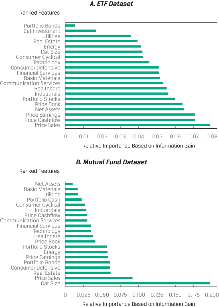
Below, you can see the results on the relative importance of the features in the random forest model for both the ETF (Panel A) and MF (Panel B) datasets. Relative importance is determined by information gain, which quantifies the amount of information that the feature holds about the response. Information gain can be regarded as a form of non-linear correlation between Y and X. Note the horizontal scale of Panel B (MF dataset) is more than twice as large as that of Panel A (ETF dataset), and the bar colors represent the feature rankings, not the features themselves.

Relative Importance of Features in the Random Forest Model

Relative Importance of Features

The prices-to-sales (price_sales) and prices-to-earnings (price_earnings) ratios are observed to be important indicators of performance, at about 0.08–0.09 and 0.06–0.07, respectively, in the random forest models for each dataset. The ratio of stocks to total assets (portfolio_stocks), at 0.06, is another key feature. Moreover, the industrials, health care, and communication services sector weightings are relatively important in the ETF dataset, while the real estate, consumer defensive, and energy sector weightings are key features in the MF dataset for differentiating between winning and losing funds.

Another important observation is that the category of the fund size (cat_size) is by far the most important feature in the model’s performance for the MF dataset (≈ 0.20), whereas it is of much less importance for model performance using the ETF dataset (≈ 0.04). Conversely, net assets is a relatively important feature for model performance using the ETF dataset (0.065), while it is the least important feature when the random forest model is applied to the MF dataset (0.01).

Conclusion

The research analyst has trained and tested machine learning–based models that she can use to identify potential winning and losing ETFs and MFs. Her classification models use input features based on fund type and size, asset class composition, fundamentals, and sector composition characteristics. She is more confident in her assessment of MFs than of ETFs, owing to the substantially larger sample size of the former. She is also confident that any imbalance in class has not led to misinterpretation of her models’ results, since she uses F1 score as her primary model evaluation metric. Moreover, she determines that the best performing model using both datasets is an ensemble-type random forest model. Finally, she concludes that while fundamental ratios, asset class ratios, and sector composition are important features for both models, net assets and category size also figure prominently in discriminating between winning and losing ETFs and MFs.