Unsupervised Machine Learning Algorithms

In this lesson, you will learn about unsupervised machine learning algorithms—including principal components analysis, K-means clustering, a...

In this lesson, you will learn about unsupervised machine learning algorithms—including principal components analysis, K-means clustering, and hierarchical clustering—and determine the problems for which they are best suited 

Unsupervised learning is machine learning that does not use labeled data (i.e., no target variable); thus, the algorithms are tasked with finding patterns within the data themselves. The two main types of unsupervised ML algorithms (displayed below) are dimension reduction, using principal components analysis, and clustering, which includes k-means and hierarchical clustering. These will now be described in turn.

Principal Components Analysis

Dimension reduction is an important type of unsupervised learning that is used widely in practice. When many features are in a dataset, representing the data visually or fitting models to the data may become extremely complex and “noisy” in the sense of reflecting random influences specific to a dataset. In such cases, dimension reduction may be necessary. Dimension reduction aims to represent a dataset with many typically correlated features by a smaller set of features that still does well in describing the data.

A long-established statistical method for dimension reduction is principal components analysis (PCA). PCA is used to summarize or transform highly correlated features of data into a few main, uncorrelated composite variables. A composite variable is a variable that combines two or more variables that are statistically strongly related to each other. Informally, PCA involves transforming the covariance matrix of the features and involves two key concepts: eigenvectors and eigenvalues. In the context of PCA, eigenvectorsdefine new, mutually uncorrelated composite variables that are linear combinations of the original features. As a vector, an eigenvector also represents a direction. Associated with each eigenvector is an eigenvalue. An eigenvalue gives the proportion of total variance in the initial data that is explained by each eigenvector. The PCA algorithm orders the eigenvectors from highest to lowest according to their eigenvalues—that is, in terms of their usefulness in explaining the total variance in the initial data (this will be shown shortly using a scree plot). PCA selects as the first principal component the eigenvector that explains the largest proportion of variation in the dataset (the eigenvector with the largest eigenvalue). The second principal component explains the next-largest proportion of variation remaining after the first principal component; this process continues for the third, fourth, and subsequent principal components. Because the principal components are linear combinations of the initial feature set, only a few principal components are typically required to explain most of the total variance in the initial feature covariance matrix.

Video here.

First and Second Principal Components of a Hypothetical Three-Dimensional Dataset

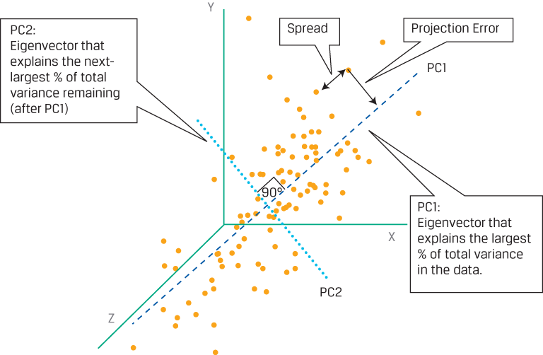
This is a hypothetical dataset with three features, so it is plotted in three dimensions along the x-, y-, and z-axes. Each data point has a measurement (x, y, z), and the data should be standardized so that the mean of each series (x’s, y’s, and z’s) is 0 and the standard deviation is 1. Assume PCA has been applied, revealing the first two principal components, PC1 and PC2. With respect to PC1, a perpendicular line dropped from each data point to PC1 shows the vertical distance between the data point and PC1, representing projection error. Moreover, the distance between each data point in the direction that is parallel to PC1 represents the spread or variation of the data along PC1. The PCA algorithm operates in such a way that it finds PC1 by selecting the line for which the sum of the projection errors for all data points is minimized and for which the sum of the spread between all the data is maximized. As a consequence of these selection criteria, PC1 is the unique vector that accounts for the largest proportion of the variance in the initial data. The next-largest portion of the remaining variance is best explained by PC2, which is at right angles to PC1 and thus is uncorrelated with PC1. The data points can now be represented by the first two principal components. This example demonstrates the effectiveness of the PCA algorithm in summarizing the variability of the data and the resulting dimension reduction.

Scree Plots

Scree Plots

It is important to know how many principal components to retain because there is a trade-off between a lower-dimensional, more manageable view of a complex dataset when a few are selected and some loss of information. Scree plots, which show the proportion of total variance in the data explained by each principal component, can be helpful in this regard (see the accompanying sidebar). In practice, the smallest number of principal components that should be retained is that which the scree plot shows as explaining a desired proportion of total variance in the initial dataset (often 85% to 95%).

Scree Plots for the Principal Components of Returns to the Hypothetical DLC 500 and VLC 30 Equity Indexes

In this illustration, researchers use scree plots and decide that three principal components are sufficient for explaining the returns to the hypothetical Diversified Large Cap (DLC) 500 and Very Large Cap (VLC) 30 equity indexes over the last 10-year period. The DLC 500 can be thought of as a diversified index of large-cap companies covering all economic sectors, while the VLC 30 is a more concentrated index of the 30 largest publicly traded companies. The dataset consists of index prices and more than 2,000 fundamental and technical features. Multi-collinearity among the features is a typical problem because that many features or combinations of features tend to have overlaps. To mitigate the problem, PCA can be used to capture the information and variance in the data. The following scree plots show that of the 20 principal components generated, the first 3 together explain about 90% and 86% of the variance in the value of the DLC 500 and VLC 30 indexes, respectively. The scree plots indicate that for each of these indexes, the incremental contribution to explaining the variance structure of the data is quite small after about the fifth principal component. Therefore, these less useful principal components can be ignored without much loss of information.

SCREE PLOTS OF PERCENT OF TOTAL VARIANCE EXPLAINED BY EACH PRINCIPAL COMPONENT FOR HYPOTHETICAL DLC 500 AND VLC 30 EQUITY INDEXES

The main drawback of PCA is that since the principal components are combinations of the dataset’s initial features, they typically cannot be easily labeled or directly interpreted by the analyst. Compared to modeling data with variables that represent well-defined concepts, the end user of PCA may perceive PCA as something of a “black box.”

Reducing the number of features to the most relevant predictors is very useful, even when working with datasets having as few as 10 or so features. Notably, dimension reduction facilitates visually representing the data in two or three dimensions. It is typically performed as part of exploratory data analysis, before training another supervised or unsupervised learning model. Machine learning models are quicker to train, tend to reduce overfitting (by avoiding the curse of dimensionality), and are easier to interpret if provided with lower-dimensional datasets.

Clustering

Clustering is another type of unsupervised machine learning, which is used to organize data points into similar groups called clusters. A cluster contains a subset of observations from the dataset such that all the observations within the same cluster are deemed “similar.” The aim is to find a good clustering of the data—meaning that the observations inside each cluster are similar or close to each other (a property known as cohesion) and the observations in two different clusters are as far away from one another or are as dissimilar as possible (a property known as separation).

Evaluating Clustering—Intra-Cluster Cohesion and Inter-Cluster Separation

Clustering algorithms are particularly useful in the many investment problems and applications in which the concept of similarity is important. Applied to grouping companies, for example, clustering may uncover important similarities and differences among companies that are not captured by standard classifications of companies by industry and sector. In portfolio management, clustering methods have been used for improving portfolio diversification.

In practice, expert human judgment has a role in using clustering algorithms. In the first place, one must establish what it means to be “similar.” Each company can be considered an observation with multiple features, including such financial statement items as total revenue and profit to shareholders, a wide array of financial ratios, or any other potential model inputs. Based on these features, a measure of similarity or “distance” between two observations (i.e., companies) can be defined. The smaller the distance, the more similar the observations; the larger the distance, the more dissimilar the observations.

A commonly used definition of distance is the Euclidian distance, the straight-line distance between two points. A closely related distance useful in portfolio diversification is correlation, which is the average Euclidian distance between a set of standardized points. Roughly a dozen different distance measures are used regularly in ML. In practice, the choice of the distance measures depends on the nature of the data (numerical or not) and the business problem being investigated. Once the relevant distance measure is defined, similar observations can be grouped together. We now introduce two of the more popular clustering approaches: k-means and hierarchical clustering.